How to Conduct Time Series Forecasting with SQL (with Example)

The future is here – for data in business, that is. As machine learning begins to take its rightful place at the forefront of data, so does predictive modeling’s prevalence in businesses. In fact, it’s almost essential for businesses to leverage predictive modeling in their operations to remain competitive in this landscape.

Why should you conduct times series forecasting?

By accurately forecasting what events will happen in the future, you can be prepared for anything that comes your way. These newly opened doors will reward you with several real-world advantages:

1. It gives you more time to strategize and execute your plan. Giving yourself more planning time allows you to refine your strategy, and ultimately, reduces the chance of error once it’s been implemented. Your future self will thank you. 🙏
2. It can help you with resource allocation. By predicting what’s trending upwards or downwards, you can allocate resources away from initiatives that are expected to have a lower ROI and move them into initiatives with higher ROIs. The bottom line? You can optimize your team’s time and set your projects up for success, so there’s more room for profits in your organization. 💰
3. It allows you to move faster than your competitors. Do you feel the need for speed? By making informed predictions about what will occur in the future, you can reassess and pivot more iteratively, allowing you to stay agile and adaptive. And yes, you can crush your competition along the way. 💪

We’re familiar with the word “forecasting” when applied in the context of “weather forecasting.” Sure, we may not necessarily be interested in the weather, but it describes the same concept: the prediction of a future trend. Although there are several types of predictive forecasting models, we’re going to focus on the popular (and valuable) model known as time series forecasting. Typically, future outcomes are completely unavailable, but using this predictive model, they can be estimated through careful time series analysis, using algorithms and evidence-based priors.

What exactly is time series forecasting?

Rather than using outliers or categories to make predictions, time series forecasting describes predictions that are made with time-stamped historical data. Can you feel the power of time-based data?!

Ok, maybe that’s an exaggeration, but in business context, there are tons of applicable use cases. Examples of time series forecasting when applied to business can actually look like:

• Predicting next month’s demand for a product to determine the amount of inventory you need.
• Estimating the number of employees who are likely to leave the company next year so you can proactively develop a hiring plan that will satisfy the company’s upcoming needs.
• Modeling the future of stock prices to determine which stock to add to the company’s portfolio.

TL;DR: the time component provides additional information that can be useful for predicting future outcomes. Adding time into the equation allows businesses to make predictions about what future events will be happening when so they can proactively plan and execute accordingly.

Depending on the complexity of your time series problem, there are a variety of techniques available to manipulate it, ranging from relatively simple visualization tools that show how trends behave to more complex machine learning models that utilize specific data set structures.

Similarly, depending on your goal, you can choose from several time series forecasting methods that have been widely adopted by the data world. For starters, there’s the autoregressive moving average model (ARMA), autoregressive integrated moving average model (ARIMA), Seasonal Autoregressive Integrated Moving-Average model (SARIMA)... and the list goes on. In this application, however, we’ll focus on the most fundamental application of stationary stochastic linear models, otherwise known as simple moving averages (SMAs).

Conducting simple time series forecasting in SQL

An SMA is a calculation that is used to forecast long-term trends using exponential smoothing; that is, taking the mean of a given metric over a specified period in the past. Super useful, right? Unfortunately, SMAs are not useful in predicting the exact future value of a metric from provided time series data. They can, however, still provide you with advantageous information based on past values.

To calculate SMAs in SQL, you’ll need two things to make up a time-series dataset:

1. A date column (or other time step column)
2. A column that represents a metric or a value that you want to forecast

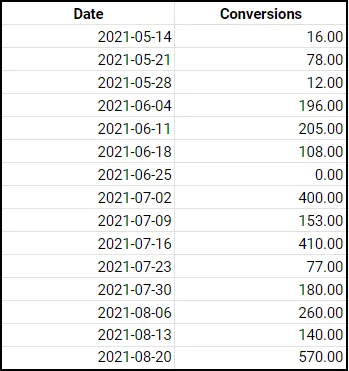
For this tutorial, let’s say we’re interested in conversions, and we have the following test set showing the number of conversions that a company had each week from May 14, 2021 to August 20, 2021.

To calculate a 7 day SMA for conversions, we could use the following code:

SELECT
Date, Conversions,
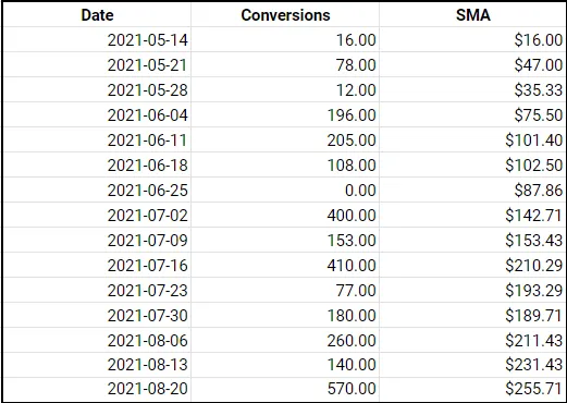
AVG(Conversions) OVER (ORDER BY Date ROWS BETWEEN 6 PRECEDING AND CURRENT ROW) as SMA
FROM daily_sales

This code would then result in the following table and chart:

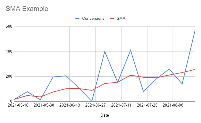
Pretty painless, right? Notice how volatile the organic conversion data (blue line) is in the chart above. In this simplified scenario, you could probably guess that conversions are trending upwards, but the raw data may not always be this intuitive for inferencing – hence the need for SMAs.

By looking at the 7-day SMA instead of the raw data:

• We can get a clear picture of a metric’s general trend. For the given conversions in this period of interest, we can see that weekly conversions are trending upwards. 📈
• We can reasonably predict where the SMA of the metric is heading. 🔮 If the most recent weekly conversion data values are above the current SMA, then the SMA should continue to trend upwards. Conversely, if conversions are consistently lower than the current SMA, we should expect it to begin to trend downward.

Voilà! Now you know how to build and interpret one of the most fundamental time-series models in SQL.

What’s next?

‍

Want to stay on the SQL train? Check out these articles next: 👇

• 5 essential SQL window functions for business operations
• Quick study guide: 5 SQL aggregate functions to use in business ops

If you’re looking to expand your knowledge base beyond SQL, you’ll find a whole collection of how-tos from the Census team here.