New to dbt? It can change your data game. | Census

I was first introduced to dbt in the second year of my data engineering career. At the time, I had no idea what it was, but I did know two things:

1. My new team was using it
2. I had to learn it quickly

It seemed like an obscure, abstract tool when others explained it to me. Unfortunately, I didn’t have someone who could explain to me exactly what dbt was in a way I could understand it. Foreign terms like targets, projects, sources, and macros were being thrown at me with no context, leaving me utterly confused, to say the least. 🙋‍♀️

But then I started experimenting with it. When I started playing around with building data models myself, I quickly realized how user-friendly it actually was. So, to share the wealth of knowledge, I want to ease you into getting to know dbt (with none of the unnecessary confusion).

We’ll start with some common misconceptions and address what dbt is not before talking about what it is, as well as the benefits it can provide to you and your team. To round this lesson out, you’ll learn how it works as we build our very own dbt model.

What dbt is not

dbt is not a new language you need to learn.

When you first hear the name dbt (or data build tool), you may think it’s some fancy, new language you need to learn. With all the hype and buzz that’s centered around dbt in the data world, you may be thinking it’s the next Python. Rest assured, dbt isn’t a new language you need to learn; it simply leverages two languages that already exist – SQL and Jinja. 😮‍💨

Jinja is usually leveraged in the more complex, macro features of dbt. For instance, you’d used Jinja in dbt configuration files where you define your database, schema, and any other information to connect to your data warehouse. It’s also leveraged in other configuration files that are a bit more specific to dbt (but we’ll save those for later).

For typical applications, dbt leverages SQL to build its models and then has its own, simple command-line functions you can use to run and compile your models. In short, if you can write a SQL query then you can use dbt.

dbt is not another costly tool to add to your data stack.

Building out a modern data stack can get expensive – fast. There’s the data warehouse itself, ingestion tools, orchestration tools, data quality monitoring tools, your data visualization platform… the list goes on.

Because these costs add up quickly, you need to make sure you’re saving costs on the right parts of your stack. Luckily, dbt is an open-source tool that is completely free to use. If you already have a data warehouse and orchestration solution in place, you only need to pay for the cost to execute dbt models in your warehouse.

dbt is not a tool that requires you to change your entire data stack.

It can be scary to add another tool to your data stack. You never know if it’s going to ruin the synchrony of your whole stack or worse, break your code. 😨

Oftentimes we stay the course much longer than we should for one, simple reason: we’re scared of change. Or, more specifically, we’re scared of disrupting the flow of the business.

Luckily, implementing dbt is nearly risk-free since it lives entirely in your data warehouse. It reads from your data warehouse and writes to it. In fact, dbt puts the T in ETL/ELT, filling that pesky transformation void you’ve been dealing with.

The transformation of your data happens all in your warehouse, making it easy to implement as long as you have raw data already in your warehouse. That means the tools that are already reading from your warehouse will function as expected, leaving you to reap the benefits of the new transformation tool.

What dbt is

Here it is, short and sweet: dbt is a data transformation tool that leverages the power of SQL and Jinja to write modular data models within your data warehouse. It reads from the data within your data warehouse and writes to it without ever leaving, allowing you to test and document your code and promoting proper code maintenance along the way.

Benefits of Using dbt

Modular data models

One of the main benefits of using dbt is that it allows you to create modular data models. What exactly does this mean? You don’t need to repeat the same SQL code over and over again in multiple models! 🥳

Have you ever had a calculation that is done in nearly every one of your models? For example, let’s say your orders, customers, and financial models all include a calculation for revenue. Instead of writing this in each of your models repetitively, you can write a single model to calculate revenue and then reference it in each model you build moving forward.

Of course, this is a fairly simple example, but this feature becomes more powerful as you adapt complex models with lots of embedded logic, saving your data analysts and analytics engineers a lot of time while keeping your code clear and easy to understand. After all, nobody likes reading thousand-line-long SQL queries.

dbt helps to keep code modular by breaking models up into two different types: staging and mart models. Staging models read directly from your raw data with a few basic transformations, while mart models are essentially the ‘final products” used by analysts and business users.

Different environments

dbt utilizes a file to create different “targets”, each with different data warehouse credentials, that contain key information like the name of your account, database, user, and password. This unique setup allows you to easily select whatever target you wish to create your data models in, making it fast and simple to run code in both development and production.

madison_project:
    target: dev
    outputs:
    	dev:
            account: 1111.us-east-2.aws
            database: data_mart_dev
            password: **
            role: transformer
            threads: 1
            type: snowflake
            user: dbt_user
            warehouse: dbt_warehouse
        prod:
            account: 11111.us-east-2.aws
            databaseL data_mart_dev
            password: **
            role: transformer
            threads: 1
            type: snowflake
            user: dbt_user
            warehouse: dbt_warehouse

Personally, when writing and testing models locally, I select the dev target; then, when I deploy my models, the orchestration tool uses the prod target. While this is how the profiles.yml file looks for setting up Snowflake, you can see examples for other data warehouses here.

Clear documentation

Perhaps one of the most underrated features of dbt is its extensive documentation features. It gives you the ability to define data models and their columns in a “source” yaml file, making it easy to keep track of key data definitions.

To make things even easier, the documentation is right beside the code itself, ensuring whoever is reading or writing the data models can see exactly what the data means. I mean, how frustrating is it to review someone's code when you have to scour through team documents to find a correct data definition? dbt cuts out the need for scouring since it keeps everything in one place.

We'll get into more of the nitty-gritty for writing a source file later in the article, but here's an example of what it looks like:

sources:
    name: adwords
    database: raw
    schema: adwords
    tables:
    	name: campaign_performance
        description: data related to the performance of campaigns in Google
        columns:
            name: campaign_id
            description: unique id of a campaign
            name: campaign_name
            description: name of a campaign
            name: campaign_status
            description: status of a campaign
            name: device
            description: device type where impression was shown
            name: campaign_date
            description: data campaign was created
            name: campaign_started_at
            description: data campaign started
            name: campaign_ended_at
            description: date campaign ended
            name: spend
            description: estimated total spent on campaign during its schedule

It contains schemas and their table names, along with the column names and definitions for each.

dbt’s documentation features give you the ability to “serve” this documentation to a user-friendly interface. Through this "data catalog" interface, you can easily see data definitions, dependencies between models, and the lineage of your entire dbt ecosystem.

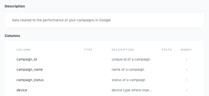
This feature is super helpful for users who aren’t familiar with dbt but need to access data definitions. It’s super easy to navigate and easy to understand – even for business users.

dbt also visualizes your lineage using a directed acyclic graph (DAG). You can see the source models (or raw data) on the left and the final mart models on the right, so each mart model can be traced back to the raw data tables that it uses.

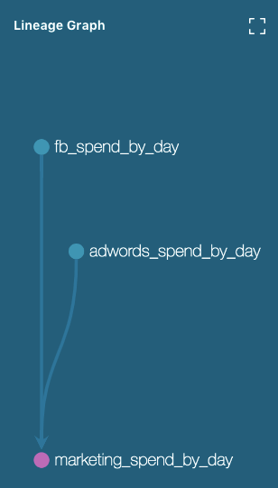
Your wishes have been granted – no more manually drawing out DAGs! Presenting data in this way also simplifies business leader conversations because it makes it easier for business users to understand the connections.

How it works

There are two key files that make dbt, well, dbt. The profiles.yml and dbt_project.yml files are unique to this transformation tool and give it a lot of power, allowing you to customize your environment to be exactly what you need. As mentioned earlier, the profiles.yml file allows you to select unique data warehouse credentials so, using different targets, you can push your data models to different databases.

The dbt_project.yml file is where you define your models. This file uses Jinja to map the paths of different models to their corresponding database and schema which is particularly helpful when you want to override what is written in the profiles.yml.

For example, it’s considered best practice to store all of your staging models as views in a different database than development or production. This way, they read directly from the raw data but don’t require everyday orchestration upkeep.

For models, I typically want to write them to a staging database rather than the development or production databases. To do this, I create a block that matches the path of my staging models under the models’ directory, and assign this to a “staging” database with a “view” materialization. This overrides whatever is set in my target.

models:
    madison_project:
    	#Config indicated by + and applies to all files under models/example
        staging:
           +materialized: view

You will want to set custom schemas here as well. Because my staging models are organized by source, I want to create a block under “staging” for each source and assign them their corresponding schema name.

models:
    madison_project:
    	#Config indicated by + and applies to all files under models/example
        staging:
           +materialized: view
           
           facebook:
              +schema: facebook

Now, all Facebook tables will be built in the “staging” database under the schema “facebook”.

Let’s build a dbt model

Now that you’ve made it through all the info, it’s time for the good stuff: building a data model that calculates total spending on ads and campaigns by the marketing team. For this purpose, we’ll be using raw data ingested from Facebook and Google Adwords.

Let’s start by building a staging model to reference our raw data sources from Facebook and Google Adwords.

Writing the staging models

Remember that staging models in dbt are reading from the source, or raw data, itself. Because of that, they should be fairly simple and contain only casting, column name changes, and simple transformations. Be sure to apply all of your data best practices such as following a naming style and casting to consistent data types!

select
    ad_id AS facebook_ad_id,
    account_id,
    ad_name,
    adset_name
    date::timestamp_ntz AS created_at,
    spend
from 

select
    campaign_id AS adwords_campaign_id,
    campaign_name AS adwords_campaign_name,
    campaign_status,
    date::timestamp_ntz AS created_at,
    start_date::timestamp_ntz AS started_at,
    end_date::timestamp_ntz AS ended_at
    cost
from 

In these models, we change some column names to make them more specific, follow a past-tense naming convention for date columns, and cast all timestamps to be timestamp_ntz. Notice that they each reference the source data which you need to define in a src.yml file, so let’s write that next!

Writing a src.yml file

Every dataset you reference using in a dbt model must be defined in a src.yml file since these read from datasets outside the dbt ecosystem. This src.yml file will live wherever the models you just defined also live. As a refresher, this is the file that populated our dbt documentation. Let’s walk through how to write this.

version: 2
sources:
    name: adwords
    database: raw
    schema: adwords
    tables:
    	name: campaign_performance
    
    name: facebook
    database: raw
    schema: facebook
    tables:
    	name: basic_ad

First, you need to fill out the name of your sources to reference within your staging models’ functions. Then, put the name of the actual database and schema of the raw data you are referencing.  In our case, we called our sources adwords and facebook and we are reading both sources from the raw database, one with a schema of adwords and the other with a schema of facebook.

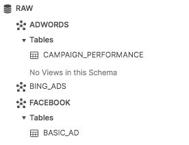
Next, write the name of the tables found in those schemas. Again, this is what you will reference in your function in your staging models, so in our case, it would be campaign_performance  and basic_ad.

For reference, here’s what this looks like in our database:

Writing the intermediate models

Now, we want to calculate the total spending for every ad and campaign on each day, for each source. We will create two intermediary models: one that calculates total spending per day for facebook and another that calculates total spending per day for adwords.

with fb_spend_summed AS (
    select
    	created_at AS spend_date,
        sum(spend) AS spend
    from 
    where spend !=0
    group by
    	created_at
)

select*from fb_spend_summed

with
adwords_spend_summed AS (
    select
    	created_at AS spend_date,
        sum(cost) AS spend
    from 
    where cost != 0
    group by
    	created_at
)

select*from adwords_spend_summed

Notice how both of these intermediary models are reading from the staging models we just built. Make sure that when you’re referencing another dbt model, you use the function with the name of the model you’re referencing inside the parenthesis.

Writing the core model

Finally, combine the results of these two models to get a model that contains the spending per day for each marketing source.

with
marketing_spend_by_day AS (
    select spend_date, spend, 'adwords' AS source from 
    UNION ALL
    select spend_date, spend, 'facebook' AS source from 
)

select*from marketing_spend_by_day

Here, we’re reading from the intermediary models we just built using the function again. We also specify the source of the spending before joining the two intermediary models.

Congrats! You’ve just built your first ever dbt data model. 🎉

Hopefully, you can see the power behind this transformation tool and how it can improve the data processes within your company. By allowing you to write modular code and document it thoroughly, dbt keeps your data environment neat and clean. ✨

There are still a ton of features you can explore on your own with dbt. For more practice, dbt has a tutorial to walk you through all the different aspects of creating a dbt project (including testing and seeds). Also, dbt offers courses to help you dive into some of the more advanced features like macros, advanced materializations, and packages. If you ever get stuck going through these resources, dbt has a Slack channel where practitioners are always answering questions on best practices and debugging your models.

The best part? You can now connect your dbt models directly with Census to streamline your sales and marketing tools! Check it out now.