Time series analysis + simple exponential smoothing in Python

You might not notice it in your daily life, but we actually rely on forecasted time series data all the time.

Have you checked tomorrow’s temperature to see if you’ll need a jacket? 🧥

Have you tried to estimate how many rolls of toilet paper you need to buy for the next month? 🧻

How about predicting the future price of your electricity bill? 🔌

All of these are examples of forecasted data in the real world. We discussed the basics in our previous article, How to conduct simple time series forecasting in SQL, but here’s a refresher: All time-series analyses involve predictions based on historical time-stamped data. As useful as it is for our day-to-day planning as individuals, it may not come as a shock that it’s just as useful for businesses, too.

In this article you’ll learn:

1. Why businesses care about forecasting
2. What exponential smoothing is
3. 3 types of exponential smoothing
4. The guiding mathematical model
5. How to perform simple exponential smoothing in Python

Why businesses care about forecasting

Let’s start with a basic business-world example: Pretend you own a business that sells products on Amazon. Obviously, it takes time for inventory to be produced and shipped, so how can you prepare how much inventory you'll need to order?  

There's really only one solution – you have to predict, or forecast, how much inventory you’ll want to produce to match demand. 🔮

Here’s the tricky part: If your company orders too much inventory and doesn’t sell it all, it loses money on the unsold merchandise – but if your company orders too little inventory, then it misses out on potential profits that it could have made if it ordered more.

This optimization problem is what makes time series forecasting so important, and this is why we’re talking about a specific time series modeling method called exponential smoothing.

What is exponential smoothing?

Exponential smoothing is one of the most widely used time series forecasting methods for univariate data, so it’s often considered a peer of (or an alternative to) the popular Box-Jenkins ARIMA class of methods for time series forecasting.

Exponential smoothing is similar to simple moving averages in the sense that it estimates future values based on past observations, but there’s a critical difference: Simple moving averages consider past observations equally, whereas exponential smoothing assigns exponentially decreasing weights over time. This means that exponential smoothing places a bigger emphasis on more recent observations, providing a weighted average.

Three types of exponential smoothing methods

There are three types of exponential smoothing models: simple exponential smoothing, double exponential smoothing, and triple exponential smoothing.

• Single (or simple) exponential smoothing is used for time-series data with no seasonality or trend. It requires a single smoothing parameter that controls the rate of influence from historical observations (indicated with a coefficient value between 0 and 1). In this technique, values closer to 1 mean that the model pays little attention to past observations, while smaller values stipulate that more of the history is taken into account during predictions.
• Double exponential smoothing is used for time-series data with no seasonality – but with a trend. This builds on the single exponential smoothing technique with an additional smoothing factor to control the influential decay of the change in trend, supporting both linear (additive) and exponential (multiplicative) trends.
• Triple exponential smoothing, also known as Holt-Winters exponential smoothing, is used for time-series data with a trend and seasonal pattern. This technique builds on the previous two techniques with a third parameter that controls the influence on the seasonal component.

Basically, each technique advances the parameters from the previous techniques to handle additional factors and provide more accurate predictions. For the rest of this article, though, we’re going to focus on single (otherwise known as simple) exponential smoothing.

Simple exponential smoothing explained

A simple exponential smoothing forecast boils down to the following equation,

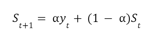
where:

• St+1 is the predicted value for the next time period
• St is the most recent predicted value
• yt is the most recent actual value
• a (alpha) is the smoothing factor between 0 and 1

In simple terms, what this equation tells us is that the predicted value for the next period (St+1) is a combination of the most recent actual value (yt) and the most recent predicted value (St).

So, why should you care about the math behind the principle? Understanding this equation gives you a better intuition in setting the alpha, yielding a more accurate prediction. 🎯

As we briefly mentioned, the smoothing factor, alpha, is the only parameter in this equation that controls the level of smoothing. When alpha is closer to 1, more emphasis is placed on the most recent actual value (so, there’s less of a smoothing effect). When alpha is closer to 0, the level of smoothing is stronger and the prediction is less sensitive to recent changes.

Ready to put it to use in Python?

Simple exponential smoothing in Python

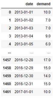
For this purpose, let’s pretend it’s January 2017 and you own a rental car agency. You’ve been open since January 1, 2013, so you have historical data on cars rented from January 1, 2013, to January 1, 2017. In this case, you have a dataset that lists the demand for all 1461 days in the 4 years you’ve been open next to its associated date, like so.

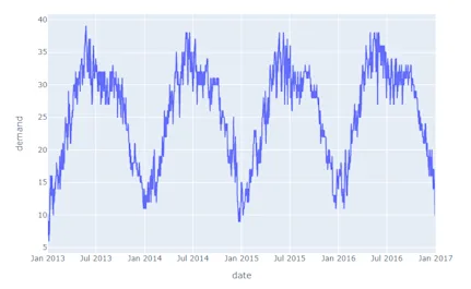
After plotting this data, you get a graph that looks something like this, with the demand plotted on the y-axis against the date:

If you wanted to forecast the number of cars that will be rented for the next week (January 2, 2017, to January 8, 2017), you could perform the time series analysis with exponential smoothing using the following steps:

Step 1. Import a method from statsmodel called SimpleExpSmoothing as well as other supporting packages.

from statsmodels.tsa.api import SimpleExpSmoothing
import pandas as pd
import plotly.express as px

Step 2. Create an instance of the class SimpleExpSmoothing (SES).

ses = SimpleExpSmoothing(df)

Step 3. Set your smoothing factor to 0.2 to take into account previous historical data.

alpha = 0.2

Step 4. Fit the model to the data as shown.

model = ses.fit(smoothing_level = alpha, optimized = False)

Step 5. Forecast the next 7 days.

forecast = model.forecast(7)

Putting that all together, your script should look like this:

from statsmodels.tsa.api import SimpleExpSmoothing
import pandas as pd
import plotly.express as px

df = pd.read_csv('data.csv')

alpha = 0.2
ses = SimpleExpSmoothing(df)
model = ses.fit(smoothing_level = alpha, optimized = False)

forecast = model.forecast(7)

After running the script and printing the output, your model gives you forecast values based on previous observations, telling you that the predicted number of cars that will be rented each day is ~15 cars.

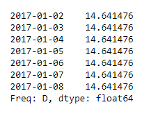
Based on this result, you could assume that over the next week you’d expect to see an average of 15 cars rented each day, allowing you and your team to prepare for this upcoming demand and keeping your customers happy.

That’s it! Pretty simple, right? Now you understand how simple exponential smoothing works, why it’s useful, and how to implement it in Python.

Want to learn more SQL? Check out these articles next: 👇

• 5 essential SQL window functions for business operations
• Quick study guide: 5 SQL aggregate functions to use in business ops

If you’re looking to expand your knowledge base beyond SQL, you’ll find a whole collection of how-tos from the Census team here.