


Two of the hottest data trends right now are machine learning and deep learning. But before you jump completely to the cutting edge, there are a variety of analytical tools and techniques that still, arguably, provide even more business value: revenue cohort analyses, marketing attribution modeling, and survival analyses.
For this piece, we’re going to focus on the last item in that list: the statistical technique of survival analysis, which determines the expected duration of time until an event occurs. We’ll take a look at what survival analysis is, its business applications, how it works, and an example of survival analysis in Python.
Let’s dive in.
What is survival analysis?
Survival analysis helps us analyze the expected duration of time before a specific event occurs. The time of an event reflects the time until something of interest happens (e.g. the occurrence of a heart attack, diagnosis of cancer, death or failure of a device, etc.).
This data analysis can help us understand our customer and product lifecycle in a variety of ways, such as predicting the cost of medical care, accessing reliability, and estimating customer life span. The collection or analysis of data begins with the occurrence of an event until failure or death and has several incredibly valuable business applications across nearly every industry.
Business applications for survival analysis in Python
As we said up top, survival analyses in Python aren’t an industry-specific technique. No matter who your customers are, what your product is, or what stack you use to support both, your team will benefit from gaining a better understanding of key metrics, such as:
- Active user survival rate
- Product time to purchase
- Campaign effectiveness evaluation
- Employee churn estimation
- Machine lifecycle measurement
Here’s a breakdown of these common use cases for survival analysis in Python.
Active user survival rate
Survival analysis can help you predict or identify customers whose survival rates (how long they’ll be active users, not a life and death thing here ☠️) are low or decreasing. This information can help you head off customer satisfaction and retention issues before their crux, and make it easier to pull together an actionable marketing strategy.
For example, if you saw that a cohort of users associated with a specific account or team type had decreasing active user survival rates (or had fully become inactive), you may check into their account usage and see that those folks aren’t getting as much of out your product as possible. Knowing this, you can have your AEs reach out to reengage those folks by showing them the features that they would get the most value out of, saving your accounts.
Product time to purchase
Survival analysis isn’t just good for understanding your customer’s activity rate. This method can also help you and your data team predict each customer’s time to purchase a product to improve your revenue forecasting.
Using survival analysis in this way can also help you predict and assess the percentage of customers that will stay subscribed to a given service over time.
Campaign effectiveness evaluation
It helps to monitor the effectiveness of a particular campaign on the survival rate so you can get a full picture of a customer’s lifetime value (LTV). Survival analysis gives you the ability to gain further insight into each of your campaign’s effectiveness.
For example, real estate and mortgage companies can leverage survival analysis to get a better understanding of time to mortgage redemption, which makes for more accurate account forecasting.
Employee churn estimation
The use cases for survival analysis in python don’t end with your customers, however. This technique can help your people ops teams gain insight into employee lifecycle and churn, too.
By calculating the survival rate for each employee (similarly to how you’d measure it for customer lifecycles), you get an estimate for how long the average employee stays with your company and can either nurture to prevent or start to prepare for departures over time.
Machine lifecycle measurement
If your company relies on machines to get things done (like pretty much any company today), survival analysis can help you predict when core components and tools will need to be replaced. Just like employee and customer lifecycle estimation, you’re measuring the time to failure for each specific machine you’re interested in.
For example, in manufacturing, companies can apply survival analysis to predict when a particular part of a process or assembly line will fail and need repair. This helps organizations avoid costly downtime and stay on top of operational health.
Math basics behind survival analysis
To understand how survival analysis works, we need to understand the basics of some core math principles. We’ll spare you a deep dive and just intuitively go over the relevant concepts below:
- Survival time
- Survival function
- Hazard function
- Kaplan-Meier method
Survival time
Survival time, denoted T, simply represents the time until an event occurs. For example, it can refer to the time until a customer churns, the time until a customer converts, or the time until a machine fails.
Survival function
The survival function, denoted as S(t), represents the probability that the event of interest has not occurred by some time t.
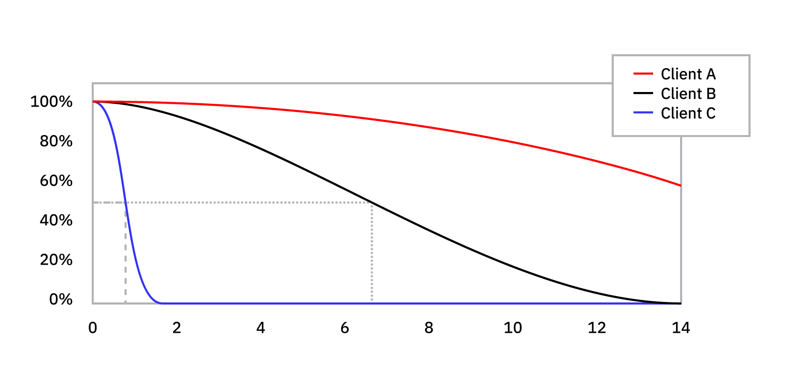
For example, by plotting the survival function for the three clients in the graphic above (known as client_A, client_B, and client_C), we know that client_C is most likely to churn before client_A and client_B. We can also tell that it’s very likely that client_C will churn in the first two weeks.
Hazard function
The hazard function, denoted at h(t), represents the conditional probability that the event will occur given that it has not occurred before. Generally, this is not the focus of survival analysis, and instead, the emphasis is on the survival function.
Kaplan-Meier method
The Kaplan-Meier method is a type of survival function that is most commonly used in applications. As shown in the survival function example above, the survival curve can help you determine a fraction of patients surviving a particular event (again, duration of accounts, not death ☠️). This involves the computation of survival probabilities from the observed event. There are three assumptions that the Kaplan-Meier method makes:
- Participants who dropped out may have the same survival prospects
- The survival probabilities will remain the same for the participants who joined late or early
- The event will occur at the specified time
To learn about the underlying mathematics behind survival analysis, check out this awesome article from Square.
Now, let’s dive into the nitty-gritty of survival analysis in python.
Coding implementation for survival analysis in Python
Python provides us with an amazing library called lifelines for survival analysis. In this demonstration, we’re using Kaplan Meier Estimation for the survival analysis. The dataset has the duration and the censoring for the heart attacks and survival of the patients.
import pandas as pd
import numpy as np
import matplotlib.pyplot as plt
import seaborn as sns
import statistics
from sklearn.impute import SimpleImputer
from lifelines import KaplanMeierFitter
from lifelines.statistics import logrank_test
fromscipy import stats
from lifelines.datasets import load_waltons
#reading data into dataframes
df=load_waltons()
#Let's assume that the preprocessing of data has been done and now implementing the Kaplan Meier method to perform survival analysis. For the sake of this analysis, let's assume that we're looking at the duration of customers until they churn.
kmp=KaplanMeierFitter()
X=df['T'] #Represents duration
Y=df['E'] #Represents whether sample was censored or not
kmp.fit(X,Y)
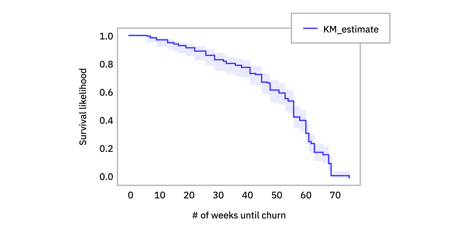
kmp.plot(). #In order to plot the survival curve
plt.xlabel(""# of weeks until churn"")
plt.ylabel(""Survival likelihood"")
plot.show()Here, we have the dataset that has a column T and E representing duration and censoring, respectively. We have applied the Kaplan Meier Estimator to our data and we plot the result. We get the following output.
Harness survival analysis in python to improve customer insights
Overall, survival analysis in python has significant value when used in the right context, such as helping you gain more insight into your customer and campaign lifecycles, as well as the longevity of your equipment. When you understand how to successfully leverage survival analysis, you can level up the insights gained into customer behavior, operations management, and marketing initiatives.
If you’re looking to further supercharge your customer data insights and operationalize your data, reach out for a 1:1 demo or start your free Census trial.