Stars, tables, and activities: How do we model the real world? | Census

For 25 years, Ralph Kimball and Margy Ross’s The Data Warehouse Toolkit has provided the mainstream method of data modeling, alternatively called Kimball-style warehouses, dimensional models, star schemas, or just “fact and dimension tables.”

In fact, it’s so ingrained in the data industry that nearly every data conference has a talk arguing for or against its continued relevance – or suggesting a new alternative altogether.

The History

For those of you who are new to the concept, fact tables are lists of events that rarely change (i.e. orders), and dimension tables are lists of entities that often change (i.e. a list of customers). To keep this straight in my mind, I often think about how a consultant once explained it to me:

You can tell what’s a fact and what’s a dimension by explaining your report with the word ‘by.’ 

Sales by customer, refunds by product, etc… it’s always fact by dimension.  Here’s an example 👇

fact_orders

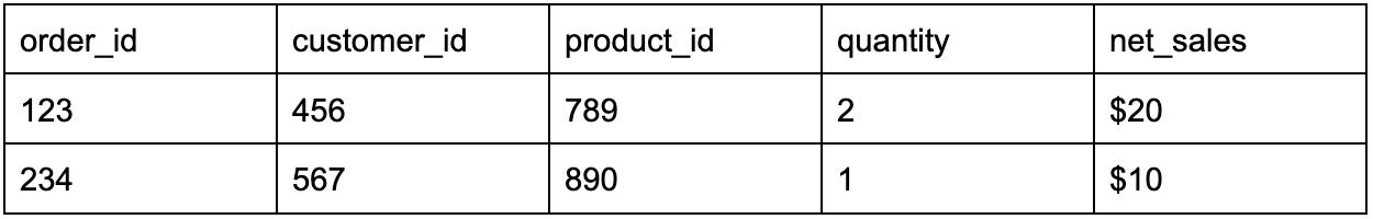
dim_customer

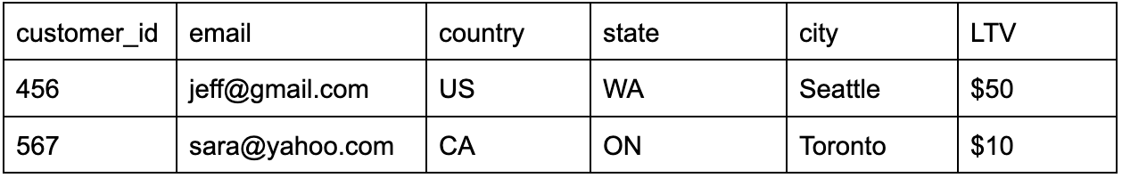
‎‎The idea here is simple: It wouldn't make sense to include the email, location, or lifetime value (LTV) of the customer on the order. Why? Those things change, and you don’t want to be updating year-old orders when your orders table has millions of rows.

The Case For Kimball

The basic organization – orders, customers, and products being separate tables – makes sense to most people. It’s easy to join the tables together and to know what to put in which table.

Even if you want to make Wide Tables, combining fact and dimensions is often the easiest way to create them, so why not make them available? Looker, for example, is well suited to dimensional models because it takes care of the joins that can make Kimball warehouses hard to navigate for business users.

But one of the main advantages of Kimball is that it provides a blueprint. 📘 I’ve worked with companies that aren’t modeling their data from ELT tools at all, and fact and dimension tables are a great model for a data warehouse. 

It’s also a common standard that new team members will be able to contribute to quickly. By comparison, if you skipped the star schema and just created Sales by Product and Sales by Customer tables, you could easily avoid problems incurred by someone asking for Sales by Customer by Product table.

The Case Against Kimball

Every modern talk about Kimball – even the ones that are generally positive – has a long list of things about Kimball that are no longer relevant to modern cloud data warehouses. 

Some of the more extreme Kimball practices (like creating a city dimension and referring to it as city ID 123 instead of the actual city name) only made sense when analytical databases were row-based and did not store repeated names efficiently. 

Plus, a huge portion of his book talks about storage costs, which are practically free nowadays. This, then, raises the question of whether dimensional modeling is an artifact of a constrained time, like how QWERTY keyboards were created to slow down typing on antiquated keyboards.

Generally, the arguments against Kimball fall into 2 main buckets:

• Business people don’t understand joins. This is the argument for Wide Tables or One Big Table, such as a table called sales_by_customer_by_product. Certain BI tools, such as Metabase, provide a good self-service interface when dealing with a single table, but are useless with star schemas.
• Separating activities into multiple fact tables makes it hard to track a user’s behavior over time. If a customer gets an email that’s in fct_email_events, visits the website which creates a few rows in fct_page_views, adds something to their cart which is recorded in fct_events, and then makes a purchase which is stored in fct_orders, it becomes hard to tell a cohesive story about why the customer made the purchase. 🤔 This is the argument for activity schemas, which combine all fact tables into a single one with a few standard columns.

Everyone has their own incentives

Tools that work well with Kimball models will suggest that you use Kimball models, while ones that do well with Wide Tables or Activity Schemas will push for those. As Aram Panasenco on dbt slack said: 

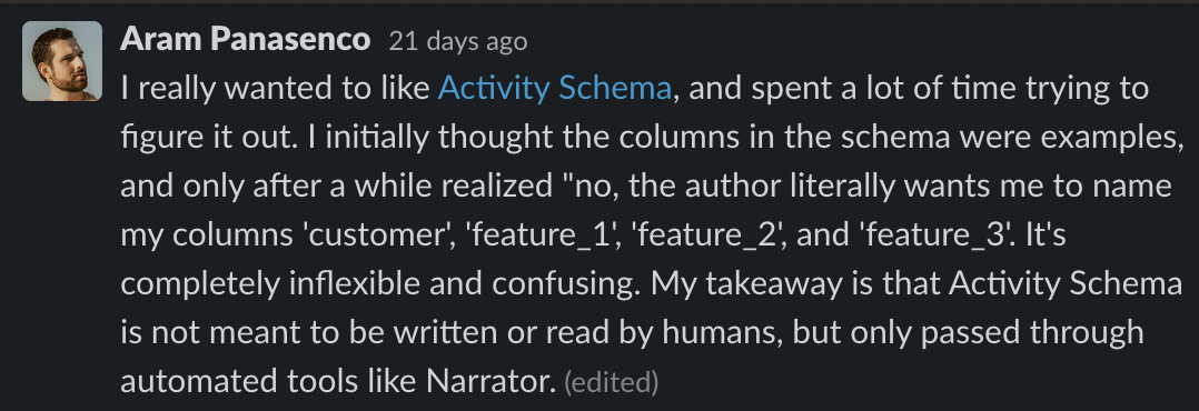
While Narrator is a cool tool — and there’s nothing wrong with implementing a schema that works well with it — you should know whether you’re implementing something for best practices or for a tool. 🧰 I’d personally love to see more discussion of giant fact tables combining all your important events (not limited to just 3 columns) that play well in a particular tool. It’s a fascinating idea!

Modern data modeling provides the answers

With modern data modeling tools like dbt, it’s very easy to create fact and dimension tables, then spin up Wide Tables as needed. Maybe your CX team wants to see Orders by Customer in Metabase, or your marketing team wants to sync Orders by Product to Salesforce with Census. Either way, it takes very little time to create views for these use cases.  

You can also create a view that turns your fact tables into a strict Activity Schema if you want to try out Narrator. Then, if you later implement Looker, you can join the fact and dimension tables directly in your Explores. Kimball modeling as the core (but not the extent) of a modern data warehouse is hard to beat in flexibility and ease of use!

👉 Want to start sending data to all your go-to-market tools to make it actionable for your teams? Book a demo with a Census product specialist.