OA Book Club Catch Up Vol. 2: Navigating the data landscape and breaking down storage needs | Census

Welcome to Volume 2 of the Operational Analytics Book Club catch-up series! If you missed the first volume, you can find that here. This article is the second part of a three-part series covering each book club meeting on The Fundamentals of Data Engineering in The OA Club (here’s more info if you’d like to join). 

Part one focused on the decision frameworks covered in the first section of the reading for our group. This second part will dive deeper into chapters 4-7, specifically looking at some of the key concepts covered around data generation, ingestion, and storage. 

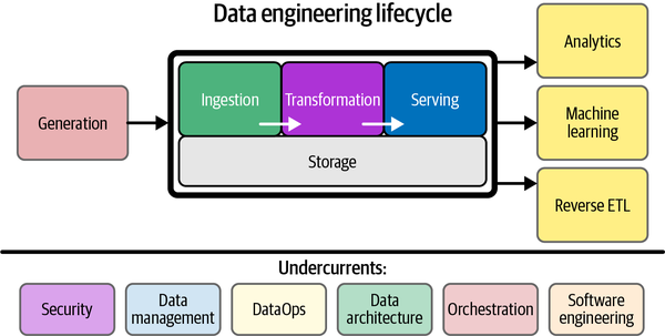
As a refresher, generation is how the data that we can use is actually created. Ingestion is the process of moving data from one location to another. Storage is the method by which we actually store all of our data.

As our book club dives further into the book, I’m consistently blown away by the authors’ ability to clearly and approachably break down complex topics and tie them back into what I see as the main theme in the books: Focus on the abstract rather than concrete tools/technologies. 

What does this theme mean? Whether you’re choosing which type of storage to use for customer order data or deciding how to move data from your lakehouse into a modeling tool, your organization will see the most success if it focuses on the value your data can create rather than specific technologies. 

Aside from more evidence for this macro principle as best practice, there were two main themes that stood out to me in the second section of the reading:  

1. The data landscape is evolving rapidly, so businesses/organizations must focus on the overcurrents of this space.
2. Business considerations need to be prioritized when selecting storage components for an organization’s data architecture, and the concept of storage is complex.

Let’s dive in! 🤓

The data landscape evolves more every day

If you ask a data engineer what the best ingestion tool will be in 10 years, they likely have no idea. New tools and technologies pop up on a daily basis; companies have more options than ever when creating their data stack. An image that took me aback is Matt Turck’s MAD (machine learning, artificial intelligence, and data) landscape. 🤯

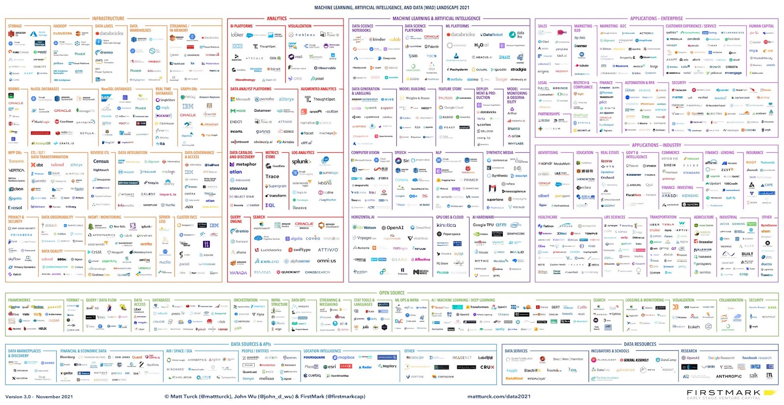
The sheer number of options available can leave any data professional feeling overwhelmed. The authors recommend evaluating tools within your data stack roughly every two years. This period of time is long enough to allow your organization to maximize the use of the tool while also remaining cognizant of other options that may prove better for your specific business need/application.

Note: Beyond just re-evaluating your stack on a regular cycle, it’s important to narrow the field of data tooling options by getting really clear on what business needs and applications you’re specifically looking to support (vs shiny window shopping from that MAD landscape). 

To drive home the point of how rapidly the data space has expanded and will continue to grow, Joe Reis and Matt Housley also broke down some of the key concepts and trends happening right now, including: 

• Containers 
• Build vs buy (everyone’s favorite debate) 

Let’s take a deeper look at these concepts.👇

Containers: One package (not one machine) to rule them all 

Containers have become “one of the most powerful trending operational technologies as of this writing. Containers play a role in both serverless and microservices” (Fundamentals of Data Engineering). You can think of containers as a type of virtual machine (VM). While traditional VMs encompass an entire operating system, containers simply encompass a single user space.

Containers arose from the common developer problem: “Well, it worked on my machine.” This became an issue because one developer would share their version of code with another developer only to find that something in the code breaks or flat out won’t run on someone else’s machine. 

Containers allow developers to package up all the necessary dependencies for a software script, which allows the code to be run on any machine without worrying about the details of said machine. There are also numerous container services that can be used. Kubernetes is one of the most popular container management systems. Kubernetes does require engineers to manage a compute cluster while AWS Fargate and Google App Engine do not. 

Build vs. buy: Is it better to have full control or free up internal resources?

One topic that frequently appears throughout the book is the argument for build versus buy. This argument simply refers to an organization’s decision to build the software required for a business need or buy the software from a vendor.

Building your own solutions gives you complete control while buying allows you to free up resources within your team and rely on others’ expertise. There are so many amazing tools already out in the world, so why not take advantage of them?

“Given the number of open source and paid services–both of which may have communities of volunteers or highly paid teams of amazing engineers–you’re foolish to build everything yourself” - Fundamentals of Data Engineering

Reis and Housley only recommend building and customizing your own solutions when it will create a competitive advantage for your business.

Does my company sit in a niche market? Do I need my tools to perform tasks that can’t be found in the market? How much time would I spend managing a custom tool?

These are all important questions to ask when deciding whether to create your own solution or buy an existing one; the financial implications also play a major role when deciding (TCO, TOCO, ROI, etc).

Data storage: The cornerstone of the data engineering lifecycle 

Many of us (including myself) take storage for granted; I had never actually taken a minute to think about how storage works until reading this book. I won’t dive too much into the nitty-gritty details, but I’ll give a quick overview of some common types: 

• Hard drives (HDD) are magnetic drives that encode binary data physically by magnetizing a film during read/write operations. 
• Solid-state drives (SSD) on the other hand store data as charges in flash memory cells, thus eliminating any mechanical means of storage. 
• Random access memory (RAM) is attached to a CPU and stores code that the CPU executes. 

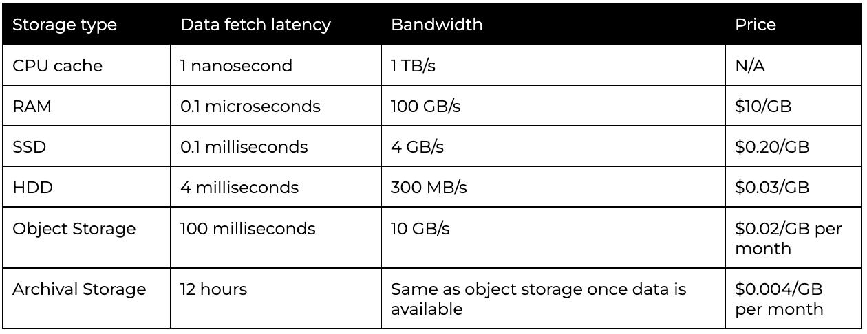
One key distinction between these types of storage is that HDD and SSD are considered nonvolatile whereas RAM is volatile. HDD and SSD tend to maintain data when powered off while RAM loses data within a second of losing power. The table below compares various types of storage and the associated costs:

‎Understanding how storage solutions inherently work will bolster your credibility as a data engineer. It is also important to consider the various types of storage systems. Here’s a further breakdown of block and object storage, each of which is used heavily in cloud-based infrastructures. 

Block storage: Ideal for frequently used, large files 

Block storage contains blocks of fixed size (4,096 bytes is standard) to store all the necessary data. Public clouds have block storage options and allow engineers to focus on storage itself rather than networking details.

Block storage in the cloud, like Amazon Elastic Block Store, creates snapshots that are frozen states of each block for backup and retrieval. After an initial backup, each snapshot is differential, which means that only blocks that have changed will be written to storage.

Given this key feature, block storage excels for large files that are regularly accessed for minor modifications. A large file would require significant computing resources to read/write each time, so using blocks allows engineers to drive computing costs down in this scenario.

Object storage: Ideal for infrequent, large data updates 

Object storage, on the other hand, contains objects; objects could be anything from a CSV file to image or video files. These are immutable, which means that after the initial write operation, they cannot support random write operations.

To update the data within an object, the object must be fully rewritten. For this reason, object storage excels at storing data that has a low frequency of updates, but when an update occurs, a large volume of data is modified. 

In summary, block storage should be used when the data in question requires a high frequency of updates but low volumes of modified data; object storage should be used when data does not need to be updated frequently, but when the data needs to be updated, a large amount is modified. 

Next up: Moving into the final stages of the DE lifecycle: ML, analytics, and more

This reading covered the early stages of the DE lifecycle necessary to find business insights from the data (i.e. generation, storage, ingestion). I’m thrilled to read about the final stages of the cycle that are more well-known among the general public: machine learning and artificial intelligence!  Again, the key topics covered in the second portion of the reading are: 

• The data engineering landscape is constantly evolving.
• Storage solutions sit at the cornerstone of the data engineering lifecycle and should be driven by creating value for your business. 

If you’re interested in joining the TitleCase OA Book Club, head to this link. Parker Rogers, data community advocate @ Census, leads it every two weeks for about an hour. It’s incredible, and I can’t emphasize just how much I’ve gained over my time in the club. I can’t wait to see you at the final Book Club meeting!